9. First Order Logic in Lean

9.1. Functions, Predicates, and Relations

In the last chapter, we discussed the language of first-order logic. We will see in the course of this book that Lean’s built-in logic is much more expressive; but it includes first-order logic, which is to say, anything that can be expressed (and proved) in first-order logic can be expressed (and proved) in Lean.

Lean is based on a foundational framework called type theory, in which every variable is assumed to range elements of some type. You can think of a type as being a “universe,” or a “domain of discourse,” in the sense of first-order logic.

For example, suppose we want to work with a first-order language with one constant symbol, one unary function symbol, one binary function symbol, one unary relation symbol, and one binary relation symbol. We can declare a new type U (for “universe”) and the relevant symbols as follows:

try it!

axiom U : Type

axiom c : U
axiom f : U → U
axiom g : U → U → U
axiom P : U → Prop
axiom R : U → U → Prop

We can then use them as follows:

try it!

variable (x y : U)

#check c
#check f c
#check g x y
#check g x (f c)

#check P (g x (f c))
#check R x y

The #check command tells us that the first four expressions have type U, and that the last two have type Prop. Roughly, this means that the first four expressions correspond to terms of first-order logic, and that the last two correspond to formulas.

Note all the following:

• A unary function is represented as an object of type U → U and a binary function is represented as an object of type U → U → U, using the same notation as for implication between propositions.

• We write, for example, f x to denote the result of applying f to x, and g x y to denote the result of applying g to x and y, again just as we did when using modus ponens for first-order logic. Parentheses are needed in the expression g x (f c) to ensure that f c is parsed as a single argument.

• A unary predicate is presented as an object of type U → Prop and a binary predicate is represented as an object of type U → U → Prop. You can think of a binary relation R as being a function that assumes two arguments in the universe, U, and returns a proposition.

• We write P x to denote the assertion that P holds of x, and R x y to denote that R holds of x and y.

You may reasonably wonder what difference there is between axiom and variable in Lean. The following declarations also work:

try it!

variable (U : Type)

variable (c : U)
variable (f : U → U)
variable (g : U → U → U)
variable (P : U → Prop)
variable (R : U → U → Prop)

variable (x y : U)

#check c
#check f c
#check g x y
#check g x (f c)

#check P (g x (f c))
#check R x y

Although the examples function in much the same way, the axiom and variable commands do very different things. The constant command declares a new object, axiomatically, and adds it to the list of objects Lean knows about. In contrast, when it is first executed, the variable command does not create anything. Rather, it tells Lean that whenever we enter an expression using the corresponding identifier, it should create a temporary variable of the corresponding type.

Many types are already declared in Lean’s standard library. For example, there is a type written Nat that denotes the natural numbers. We can introduce notation ℕ for it.

try it!

#check Nat

notation:1 "ℕ" => Nat

#check ℕ

You can enter the unicode ℕ with \nat or \N. The two expressions mean the same thing.

Using this built-in type, we can model the language of arithmetic, as described in the last chapter, as follows:

try it!

namespace hidden
notation:1 "ℕ" => Nat

axiom mul : ℕ → ℕ → ℕ
axiom add : ℕ → ℕ → ℕ
axiom square : ℕ → ℕ
axiom even : ℕ → Prop
axiom odd : ℕ → Prop
axiom prime : ℕ → Prop
axiom divides : ℕ → ℕ → Prop
axiom lt : ℕ → ℕ → Prop
axiom zero : ℕ
axiom one : ℕ

end hidden

We have used the namespace command to avoid conflicts with identifiers that are already declared in the Lean library. (Outside the namespace, the constant mul we just declared is named hidden.mul.) We can again use the #check command to try them out:

try it!

namespace hidden

variable (w x y z : ℕ)

#check mul x y
#check add x y
#check square x
#check even x

end hidden

We can even declare infix notation of binary operations and relations:

try it!

local infix:65   " + " => add
local infix:70   " * " => mul
local infix:50   " < " => lt

(Getting notation for numerals 1, 2, 3, … is trickier.) With all this in place, the examples above can be rendered as follows:

try it!

#check even (x + y + z) ∧ prime ((x + one) * y * y)
#check ¬ (square (x + y * z) = w) ∨ x + y < z
#check x < y ∧ even x ∧ even y → x + one < y

In fact, all of the functions, predicates, and relations discussed here, except for the “square” function, are defined in the Lean library. They become available to us when we import the module import Mathlib.Data.Nat.Prime at the top of a file.

try it!

import Mathlib.Data.Nat.Prime

axiom square : ℕ → ℕ

variable (w x y z : ℕ)

#check Even (x + y + z) ∧ Prime ((x + 1) * y * y)
#check ¬ (square (x + y * z) = w) ∨ x + y < z
#check x < y ∧ Even x ∧ Even y → x + 1 < y

Here, we declare the constant square axiomatically, but refer to the other operations and predicates in the Lean library. In this book, we will often proceed in this way, telling you explicitly what facts from the library you should use for exercises.

Again, note the following aspects of syntax:

• In contrast to ordinary mathematical notation, in Lean, functions are applied without parentheses or commas. For example, we write square x and add x y instead of \(\mathit{square}(x)\) and \(\mathit{add}(x, y)\).

• The same holds for predicates and relations: we write even x and lt x y instead of \(\mathit{even}(x)\) and \(\mathit{lt}(x, y)\), as one might do in symbolic logic.

• The notation add : ℕ → ℕ → ℕ indicates that addition assumes two arguments, both natural numbers, and returns a natural number.

• Similarly, the notation divides : ℕ → ℕ → Prop indicates that divides is a binary relation, which assumes two natural numbers as arguments and forms a proposition. In other words, divides x y expresses the assertion that x divides y.

Lean can help us distinguish between terms and formulas. If we #check the expression x + y + 1 in Lean, we are told it has type ℕ, which is to say, it denotes a natural number. If we #check the expression even (x + y + 1), we are told that it has type Prop, which is to say, it expresses a proposition.

In Chapter 7 we considered many-sorted logic, where one can have multiple universes. For example, we might want to use first-order logic for geometry, with quantifiers ranging over points and lines. In Lean, we can model this as by introducing a new type for each sort:

try it!

variable (Point Line : Type)
variable (lies_on : Point → Line → Prop)

We can then express that two distinct points determine a line as follows:

try it!

#check ∀ (p q : Point) (L M : Line),
        p ≠ q → lies_on p L → lies_on q L → lies_on p M →
          lies_on q M → L = M

Notice that we have followed the convention of using iterated implication rather than conjunction in the antecedent. In fact, Lean is smart enough to infer what sorts of objects p, q, L, and M are from the fact that they are used with the relation lies_on, so we could have written, more simply, this:

try it!

#check ∀ p q L M, p ≠ q → lies_on p L → lies_on q L →
  lies_on p M → lies_on q M → L = M

9.2. Using the Universal Quantifier

In Lean, you can enter the universal quantifier by writing \all. The motivating examples from Section 7.1 are rendered as follows:

try it!

import Mathlib.Data.Nat.Prime

#check ∀ x, (Even x ∨ Odd x) ∧ ¬ (Even x ∧ Odd x)
#check ∀ x, Even x ↔ 2 ∣ x
#check ∀ x, Even x → Even (x^2)
#check ∀ x, Even x ↔ Odd (x + 1)
#check ∀ x, Prime x ∧ x > 2 → Odd x
#check ∀ x y z, x ∣ y → y ∣ z → x ∣ z

Remember that Lean expects a comma after the universal quantifier, and gives it the widest scope possible. For example, ∀ x, P ∨ Q is interpreted as ∀ x, (P ∨ Q), and we would write (∀ x, P) ∨ Q to limit the scope. If you prefer, you can use the plain ascii expression forall instead of the unicode ∀.

In Lean, then, the pattern for proving a universal statement is rendered as follows:

try it!

variable (U : Type)
variable (P : U → Prop)

example : ∀ x, P x :=
fun x ↦
show P x from sorry

Read fun x as “fix an arbitrary value x of U.” Since we are allowed to rename bound variables at will, we can equivalently write either of the following:

try it!

variable (U : Type)
variable (P : U → Prop)

example : ∀ y, P y :=
fun x ↦
show P x from sorry

example : ∀ x, P x :=
fun y ↦
show P y from sorry

This constitutes the introduction rule for the universal quantifier. It is very similar to the introduction rule for implication: instead of using fun to temporarily introduce an assumption, we use fun to temporarily introduce a new object, y. (In fact, both are alternate syntax for a single internal construct in Lean, which can also be denoted by λ.)

The elimination rule is, similarly, implemented as follows:

try it!

variable (U : Type)
variable (P : U → Prop)
variable (h : ∀ x, P x)
variable (a : U)

example : P a :=
show P a from h a

Observe the notation: P a is obtained by “applying” the hypothesis h to a. Once again, note the similarity to the elimination rule for implication.

Here is an example of how it is used:

try it!

variable (U : Type)
variable (A B : U → Prop)

example (h1 : ∀ x, A x → B x) (h2 : ∀ x, A x) : ∀ x, B x :=
fun y ↦
have h3 : A y := h2 y
have h4 : A y → B y := h1 y
show B y from h4 h3

Here is an even shorter version of the same proof, where we avoid using have:

try it!

example (h1 : ∀ x, A x → B x) (h2 : ∀ x, A x) : ∀ x, B x :=
fun y ↦
show B y from h1 y (h2 y)

You should talk through the steps, here. Applying h1 to y yields a proof of A y → B y, which we then apply to h2 y, which is a proof of A y. The result is the proof of B y that we are after.

In the last chapter, we considered the following proof in natural deduction:

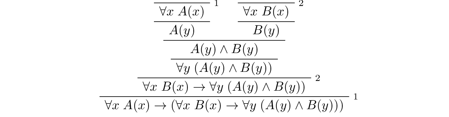
Here is the same proof rendered in Lean:

try it!

variable (U : Type)
variable (A B : U → Prop)

example : (∀ x, A x) → (∀ x, B x) → (∀ x, A x ∧ B x) :=
fun hA : ∀ x, A x ↦
  fun hB : ∀ x, B x ↦
    fun y ↦
      have Ay : A y := hA y
      have By : B y := hB y
      show A y ∧ B y from And.intro Ay By

Here is an alternative version, using the “anonymous” versions of have:

try it!

example : (∀ x, A x) → (∀ x, B x) → (∀ x, A x ∧ B x) :=
fun hA : ∀ x, A x ↦
  fun hB : ∀ x, B x ↦
    fun y ↦
      have : A y := hA y
      have : B y := hB y
      show A y ∧ B y from And.intro ‹A y› ‹B y›

The exercises below ask you to prove the barber paradox, which was discussed in the last chapter. You can do that using only propositional reasoning and the rules for the universal quantifier that we have just discussed.

9.3. Using the Existential Quantifier

In Lean, you can type the existential quantifier, ∃, by writing \ex. If you prefer you can use the ascii equivalent, Exists. The introduction rule is Exists.intro and requires two arguments: a term, and a proof that term satisfies the required property.

try it!

variable (U : Type)
variable (P : U → Prop)

example (y : U) (h : P y) : ∃ x, P x :=
Exists.intro y h

The elimination rule for the existential quantifier is given by Exists.elim. It follows the form of the natural deduction rule: if we know ∃x, P x and we are trying to prove Q, it suffices to introduce a new variable, y, and prove Q under the assumption that P y holds.

try it!

variable (U : Type)
variable (P : U → Prop)
variable (Q : Prop)

example (h1 : ∃ x, P x) (h2 : ∀ x, P x → Q) : Q :=
Exists.elim h1
  (fun (y : U) (h : P y) ↦
  have h3 : P y → Q := h2 y
  show Q from h3 h)

As usual, we can leave off the information as to the data type of y and the hypothesis h after the fun, since Lean can figure them out from the context. Deleting the show and replacing h3 by its proof, h2 y, yields a short (though virtually unreadable) proof of the conclusion.

try it!

example (h1 : ∃ x, P x) (h2 : ∀ x, P x → Q) : Q :=
Exists.elim h1
  (fun y h ↦ h2 y h)

The following example uses both the introduction and the elimination rules for the existential quantifier.

try it!

variable (U : Type)
variable (A B : U → Prop)

example : (∃ x, A x ∧ B x) → ∃ x, A x :=
fun h1 : ∃ x, A x ∧ B x ↦
Exists.elim h1
  (fun y (h2 : A y ∧ B y) ↦
  have h3 : A y := And.left h2
  show ∃ x, A x from Exists.intro y h3)

Notice the parentheses in the hypothesis; if we left them out, everything after the first ∃ x would be included in the scope of that quantifier. From the hypothesis, we obtain a y that satisfies A y ∧ B y, and hence A y in particular. So y is enough to witness the conclusion.

It is sometimes annoying to enclose the proof after an Exists.elim in parenthesis, as we did here with the fun ... show block. To avoid that, we can use a bit of syntax from the programming world, and use a dollar sign instead. In Lean, an expression f $ t means the same thing as f (t), with the advantage that we do not have to remember to close the parenthesis. With this gadget, we can write the proof above as follows:

try it!

example : (∃ x, A x ∧ B x) → ∃ x, A x :=
fun h1 : ∃ x, A x ∧ B x ↦
Exists.elim h1 $
fun y (h2 : A y ∧ B y) ↦
have h3 : A y := And.left h2
show ∃ x, A x from ⟨y, h3⟩

Like with And.intro, we can use the use \< and \> as syntax for Exists.intro, which we used in the last line of the example above.

The following example is more involved:

try it!

example : (∃ x, A x ∨ B x) → (∃ x, A x) ∨ (∃ x, B x) :=
fun h1 : ∃ x, A x ∨ B x ↦
Exists.elim h1 $
fun y (h2 : A y ∨ B y) ↦
Or.elim h2
  (fun h3 : A y ↦
    have h4 : ∃ x, A x := Exists.intro y h3
    show (∃ x, A x) ∨ (∃ x, B x) from Or.inl h4)
  (fun h3 : B y ↦
    have h4 : ∃ x, B x := Exists.intro y h3
    show (∃ x, A x) ∨ (∃ x, B x) from Or.inr h4)

Note again the placement of parentheses in the statement.

In the last chapter, we considered the following natural deduction proof:

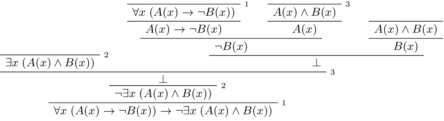
Here is a proof of the same implication in Lean:

try it!

variable (U : Type)
variable (A B : U → Prop)

example : (∀ x, A x → ¬ B x) → ¬ ∃ x, A x ∧ B x :=
fun h1 : ∀ x, A x → ¬ B x ↦
fun h2 : ∃ x, A x ∧ B x ↦
Exists.elim h2 $
fun x (h3 : A x ∧ B x) ↦
have h4 : A x := And.left h3
have h5 : B x := And.right h3
have h6 : ¬ B x := h1 x h4
show False from h6 h5

Here, we use Exists.elim to introduce a value x satisfying A x ∧ B x. The name is arbitrary; we could just as well have used z:

try it!

example : (∀ x, A x → ¬ B x) → ¬ ∃ x, A x ∧ B x :=
fun h1 : ∀ x, A x → ¬ B x ↦
fun h2 : ∃ x, A x ∧ B x ↦
Exists.elim h2 $
fun z (h3 : A z ∧ B z) ↦
have h4 : A z := And.left h3
have h5 : B z := And.right h3
have h6 : ¬ B z := h1 z h4
show False from h6 h5

Here is another example of the exists-elimination rule:

try it!

variable (U : Type)
variable (u : U)
variable (P : Prop)

example : (∃x : U, P) ↔ P :=
Iff.intro
  (fun h1 : ∃x, P ↦
    Exists.elim h1 $
    fun x (h2 : P) ↦
    h2)
  (fun h1 : P ↦
    ⟨u, h1⟩)

This is subtle: the proof does not go through if we do not declare a variable u of type U, even though u does not appear in the statement of the theorem. This highlights a difference between first-order logic and the logic implemented in Lean. In natural deduction, we can prove \(\forall x \; P(x) \to \exists x \; P(x)\), which shows that our proof system implicitly assumes that the universe has at least one object. In contrast, the statement (∀ x : U, P x) → ∃ x : U, P x is not provable in Lean. In other words, in Lean, it is possible for a type to be empty, and so the proof above requires an explicit assumption that there is an element u in U.

9.4. Equality

In Lean, reflexivity, symmetry, and transitivity are called Eq.refl, Eq.symm, and Eq.trans, and the second substitution rule is called Eq.subst. Their uses are illustrated below.

try it!

variable (A : Type)

variable (x y z : A)
variable (P : A → Prop)

example : x = x :=
show x = x from Eq.refl x

example : y = x :=
have h : x = y := sorry
show y = x from Eq.symm h

example : x = z :=
have h1 : x = y := sorry
have h2 : y = z := sorry
show x = z from Eq.trans h1 h2

example : P y :=
have h1 : x = y := sorry
have h2 : P x := sorry
show P y from Eq.subst h1 h2

The rule Eq.refl above assumes x as an argument, because there is no hypothesis to infer it from. All the other rules assume their premises as arguments. Here is an example of equational reasoning:

try it!

variable (A : Type) (x y z : A)

example : y = x → y = z → x = z :=
fun h1 : y = x ↦
fun h2 : y = z ↦
have h3 : x = y := Eq.symm h1
show x = z from Eq.trans h3 h2

This proof can be written more concisely:

try it!

example : y = x → y = z → x = z :=
fun h1 h2 ↦ Eq.trans (Eq.symm h1) h2

9.5. Tactic Mode

9.5.1. Universal quantifiers

Just like for conditionals, in tactic mode we can also use intro x to introduce a variable, or “fix an arbitrary value x : U”. This would change the goal from ∀ x, A x to A x. Conversely when we have a proof h : ∀ x, A x of a universal quantifier, and our goal is A a for some a : U, we can use apply h to close the goal. Here is the example from earlier in tactic mode:

try it!

example (h1 : ∀ x, A x → B x) (h2 : ∀ x, A x) : ∀ x, B x := by
  intro y
  have h3 : A y → B y := by apply h1
  show B y
  apply h3
  show A y
  apply h2

The tactic apply can combine hypothesis and only require us to provide those that remain. For example, if we were to immediately do apply h1 when showing B y Lean would recognize that we need to supply y in place of x and then ask us to show A y.

try it!

example (h1 : ∀ x, A x → B x) (h2 : ∀ x, A x) : ∀ x, B x := by
  intro y
  show B y
  apply h1
  show A y
  apply h2

9.5.2. Existential quantifiers

Recall the example

try it!

example : (∃ x, A x ∧ B x) → ∃ x, A x :=
fun h1 : ∃ x, A x ∧ B x ↦
Exists.elim h1 $
fun y (h2 : A y ∧ B y) ↦
have h3 : A y := And.left h2
show ∃ x, A x from Exists.intro y h3

In tactic mode we could prove this in the following way

try it!

example : (∃ x, A x ∧ B x) → ∃ x, A x := by
  intro (h1 : ∃ x, A x ∧ B x)
  cases h1 with
  | intro y h2 =>
    show ∃ x, A x
    apply Exists.intro y
    show A x
    cases h2 with
    | intro h3 _ =>
      exact h3

By doing cases h1 we obtain only one possible case for how a proof h1 : ∃ x, A x ∧ B x was constructed - namely by Exists.intro y h2 where y : U and h2 : A y ∧ B y (Lean’s syntax omits the Exists.). Given a y : U, Lean sees Exists.intro y : A y → ∃ x, A x as a conditional. So we can use apply Exists.intro y to change the goal from A x to ∃ x, A x.

A further example from before

try it!

-- term mode
example : (∃ x, A x ∨ B x) → (∃ x, A x) ∨ (∃ x, B x) :=
fun h1 : ∃ x, A x ∨ B x ↦
Exists.elim h1 $
fun y (h2 : A y ∨ B y) ↦
Or.elim h2
  (fun h3 : A y ↦
    have h4 : ∃ x, A x := Exists.intro y h3
    show (∃ x, A x) ∨ (∃ x, B x) from Or.inl h4)
  (fun h3 : B y ↦
    have h4 : ∃ x, B x := Exists.intro y h3
    show (∃ x, A x) ∨ (∃ x, B x) from Or.inr h4)

-- tactic mode
example : (∃ x, A x ∨ B x) → (∃ x, A x) ∨ (∃ x, B x) := by
  intro (h1 : ∃ x, A x ∨ B x)
  cases h1 with
  | intro y h2 =>
    cases h2 with
    | inl h3 =>
      show (∃ x, A x) ∨ (∃ x, B x)
      apply Or.inl
      show (∃ x, A x)
      apply Exists.intro y
      exact h3
    | inr h3 =>
      show (∃ x, A x) ∨ (∃ x, B x)
      apply Or.inr
      show (∃ x, B x)
      apply Exists.intro y
      exact h3

-- term-tactic mix
example : (∃ x, A x ∨ B x) → (∃ x, A x) ∨ (∃ x, B x) := by
  intro (h1 : ∃ x, A x ∨ B x)
  cases h1 with
  | intro y h2 =>
    cases h2 with
    | inl h3 => exact Or.inl (Exists.intro y h3)
    | inr h3 => exact Or.inr (Exists.intro y h3)

If we don’t want to present our proof backwards using apply, we might opt for the style of our final example above, returning to term mode after breaking down the assumption h1 completely.

The obtain tactic provides us an alternative to cases for eliminating existentials. Again, we take a proof h1 : ∃ y, P y of an extenstential and break it up into a pair ⟨x, (h2 : P x)⟩ := h1. It can also do nested eliminations, so that the second proof below is just a shorter version of the first:

try it!

variable (U : Type) (R : U → U → Prop)

example : (∃ x, ∃ y, R x y) → (∃ y, ∃ x, R x y) := by
intro (h1 : ∃ x, ∃ y, R x y)
obtain ⟨x, (h2 : ∃ y, R x y)⟩ := h1
obtain ⟨y, (h3 : R x y)⟩ := h2
apply Exists.intro y
apply Exists.intro x
exact h3

example : (∃ x, ∃ y, R x y) → (∃ y, ∃ x, R x y) := by
intro (h1 : ∃ x, ∃ y, R x y)
obtain ⟨x, ⟨y, (h3 : R x y)⟩⟩ := h1
exact ⟨y, ⟨x, h3⟩⟩

You can also use obtain to extract the components of an “and”:

try it!

variable (A B : Prop)

example : A ∧ B → B ∧ A := by
intro (h1 : A ∧ B)
obtain ⟨(h2 : A), (h3 : B) ⟩ := h1
show B ∧ A
exact ⟨h3, h2⟩

9.5.3. Equality

Because calculations are so important in mathematics, Lean provides more efficient ways of carrying them out. One method is to use the `rewrite tactic, which carries out substitutions along equalities on parts of the goal.

Recall the example

try it!

example : y = x → y = z → x = z :=
fun h1 h2 ↦ Eq.trans (Eq.symm h1) h2

A tactic mode proof of this would look like:

try it!

example : y = x → y = z → x = z := by
  intro (hyx : y = x) (hyz : y = z)
  rewrite [←hyx]
  exact hyz

If you put the cursor before rewrite, Lean will tell you that the goal at that point is to prove x = z. The first command changes the goal x = z to y = z; the left-facing arrow before hyx (which you can enter as \<-) tells Lean to use the equation in the reverse direction. If you put the cursor before exact Lean shows you the new goal, y = z. The apply command uses hyz to complete the proof.

An alternative is to rewrite the goal using hyx and hyz, which reduces the goal to x = x. When that happens, rewrite automatically applies reflexivity. Rewriting is such a common operation in Lean that we can use the shorthand rw in place of the full rewrite.

try it!

example : y = x → y = z → x = z := by
  intro (hyx : y = x) (hyz : y = z)
  rw [←hyx]
  rw [hyz]

In fact, a sequence of rewrites can be combined, using square brackets:

try it!

example : y = x → y = z → x = z := by
  intro (hyx : y = x) (hyz : y = z)
  rw [←hyx, hyz]

try it!

example : y = x → y = z → x = z :=
assume h1 : y = x,
assume h2 : y = z,
show x = z, by rw [←h1, h2]

If you put the cursor after the ←h1, Lean shows you the goal at that point.

The tactic rewrite can also be used for substituting along biconditionals. For example, if our goal were A ∧ B but we know that hAC : A ↔ C and C ∧ B, then we could rewrite A for C using hAC, changing out goal to C ∧ B.

try it!

example (hAC : A ↔ C) (hCB : C ∧ B) : A ∧ B := by
  rw [hAC]
  exact hCB

In the following example we use an Iff lemma from Mathlib and the fact that 1 is odd to show that 1 is not even.

try it!

import Mathlib.Data.Nat.Prime
open Nat

#check odd_iff_not_even
#check odd_one

example : ¬ Even 1 := by
  rw [← odd_iff_not_even]
  exact odd_one

9.6. Calculational Proofs

We will see in the coming chapters that in ordinary mathematical proofs, one commonly carries out calculations in a format like this:

\[\begin{split}t_1 &= t_2 \\ \ldots & = t_3 \\ \ldots &= t_4 \\ \ldots &= t_5.\end{split}\]

Lean has a mechanism to model such calculational proofs. Whenever a proof of an equation is expected, you can provide a proof using the identifier calc, following by a chain of equalities and justification, in the following form:

calc
  e1 = e2 := justification 1
   _ = e3 := justification 2
   _ = e4 := justification 3
   _ = e5 := justification 4

The chain can go on as long as needed, and in this example the result is a proof of e1 = e5. Each justification is the name of the assumption or theorem that is used. For example, the previous proof could be written as follows:

try it!

example : y = x → y = z → x = z :=
fun h1 : y = x ↦
fun h2 : y = z ↦
calc
  x = y := Eq.symm h1
  _ = z := h2

As usual, the syntax is finicky; notice that there are no commas in the calc expression, and the := and underscores must be in the correct form. It is also sensitive to whitespace All that varies are the expressions e1, e2, e3, ... and the justifications themselves.

The calc environment is most powerful when used in conjunction with rewrite, since we can then rewrite expressions with facts from the library. For example, Lean’s library has a number of basic identities for the integers, such as these:

try it!

import Mathlib.Data.Int.Defs

variable (x y z : Int)

example : x + 0 = x :=
Int.add_zero x

example : 0 + x = x :=
Int.zero_add x

example : (x + y) + z = x + (y + z) :=
Int.add_assoc x y z

example : x + y = y + x :=
Int.add_comm x y

example : (x * y) * z = x * (y * z) :=
Int.mul_assoc x y z

example : x * y = y * x :=
Int.mul_comm x y

example : x * (y + z) = x * y + x * z :=
Int.mul_add x y z

example : (x + y) * z = x * z + y * z :=
Int.add_mul x y z

You can also write the type of integers as ℤ, entered with either \Z or \int. We have imported the file Mathlib.Data.Int.Defs to make all the basic properties of the integers available to us. (In later snippets, we will suppress this line in the online and pdf versions of the textbook, to avoid clutter.) Notice that, for example, Int.add_comm is the theorem ∀ x y, x + y = y + x. So to instantiate it to s + t = t + s, you write Int.add_comm s t. Using these axioms, here is the calculation above rendered in Lean, as a theorem about the integers:

try it!

example (x y z : Int) : (x + y) + z = (x + z) + y :=
calc
      (x + y) + z
    = x + (y + z) := Int.add_assoc x y z
  _ = x + (z + y) := @Eq.subst _ (λ w ↦ x + (y + z) = x + w) _ _ (Int.add_comm y z) rfl
  _ = (x + z) + y := Eq.symm (Int.add_assoc x z y)

We had to use @ on Eq.subst to fill in some of the implicit arguments, because the provided information was insufficient. Using rewrite simplifies the work, though at times we have to provide information to specify where the rules are used:

try it!

example (x y z : Int) : (x + y) + z = (x + z) + y :=
calc
  (x + y) + z = x + (y + z) := by rw [Int.add_assoc]
          _ = x + (z + y) := by rw [Int.add_comm y z]
          _ = (x + z) + y := by rw [Int.add_assoc]

In this case, we can use a single rewrite:

try it!

example (x y z : Int) : (x + y) + z = (x + z) + y :=
by rw [Int.add_assoc, Int.add_comm y z, Int.add_assoc]

Here is another example:

try it!

variable (a b d c : Int)

example : (a + b) * (c + d) = a * c + b * c + a * d + b * d :=
calc
  (a + b) * (c + d) = (a + b) * c + (a + b) * d := by rw [Int.mul_add]
    _ = (a * c + b * c) + (a + b) * d         := by rw [Int.add_mul]
    _ = (a * c + b * c) + (a * d + b * d)     := by rw [Int.add_mul]
    _ = a * c + b * c + a * d + b * d         := by rw [←Int.add_assoc]

Once again, there is a shorter proof:

try it!

variable (a b d c : Int)

example : (a + b) * (c + d) = a * c + b * c + a * d + b * d :=
by rw [Int.mul_add, Int.add_mul, Int.add_mul, ←Int.add_assoc]

9.7. Exercises

1. Fill in the sorry in term mode.

   try it!

   section
     variable (A : Type)
     variable (f : A → A)
     variable (P : A → Prop)
     variable (h : ∀ x, P x → P (f x))
   
     -- Show the following:
     example : ∀ y, P y → P (f (f y)) :=
     sorry
   end
   

2. Fill in the sorry in tactic mode.

   try it!

   section
     variable (U : Type)
     variable (A B : U → Prop)
   
     example : (∀ x, A x ∧ B x) → ∀ x, A x := by
     sorry
   end
   

3. Fill in the sorry (assume that this means in your preferred style, unless specified otherwise).

   try it!

   section
     variable (U : Type)
     variable (A B C : U → Prop)
   
     variable (h1 : ∀ x, A x ∨ B x)
     variable (h2 : ∀ x, A x → C x)
     variable (h3 : ∀ x, B x → C x)
   
     example : ∀ x, C x :=
     sorry
   end
   

4. Fill in the sorry’s below, to prove the barber paradox.

   try it!

   open Classical   -- not needed, but you can use it
   
   -- This is an exercise from Chapter 4. Use it as an axiom here.
   axiom not_iff_not_self (P : Prop) : ¬ (P ↔ ¬ P)
   
   example (Q : Prop) : ¬ (Q ↔ ¬ Q) :=
   not_iff_not_self Q
   
   section
     variable (Person : Type)
     variable (shaves : Person → Person → Prop)
     variable (barber : Person)
     variable (h : ∀ x, shaves barber x ↔ ¬ shaves x x)
   
     -- Show the following:
     example : False :=
     sorry
   end
   

5. Fill in the sorry.

   try it!

   section
     variable (U : Type)
     variable (A B : U → Prop)
   
     example : (∃ x, A x) → ∃ x, A x ∨ B x :=
     sorry
   end
   

6. Fill in the sorry.

   try it!

   section
     variable (U : Type)
     variable (A B : U → Prop)
   
     variable (h1 : ∀ x, A x → B x)
     variable (h2 : ∃ x, A x)
   
     example : ∃ x, B x :=
     sorry
   end
   

7. Fill in the sorry.

   try it!

   variable (U : Type)
   variable (A B C : U → Prop)
   
   example (h1 : ∃ x, A x ∧ B x) (h2 : ∀ x, B x → C x) :
       ∃ x, A x ∧ C x :=
   sorry
   

8. Complete these proofs.

   try it!

   variable (U : Type)
   variable (A B C : U → Prop)
   
   example : (¬ ∃ x, A x) → ∀ x, ¬ A x :=
   sorry
   
   example : (∀ x, ¬ A x) → ¬ ∃ x, A x :=
   sorry
   

9. Fill in the sorry.

   try it!

   variable (U : Type)
   variable (R : U → U → Prop)
   
   example : (∃ x, ∀ y, R x y) → ∀ y, ∃ x, R x y :=
   sorry
   

10. The following exercise shows that in the presence of reflexivity, the rules for symmetry and transitivity are equivalent to a single rule.

    try it!

    theorem foo {A : Type} {a b c : A} : a = b → c = b → a = c :=
    sorry
    
    -- notice that you can now use foo as a rule. The curly braces mean that
    -- you do not have to give A, a, b, or c
    
    section
      variable (A : Type)
      variable (a b c : A)
    
      example (h1 : a = b) (h2 : c = b) : a = c :=
      foo h1 h2
    end
    
    section
      variable {A : Type}
      variable {a b c : A}
    
      -- replace the sorry with a proof, using foo and rfl, without using eq.symm.
      theorem my_symm (h : b = a) : a = b :=
      sorry
    
      -- now use foo and my_symm to prove transitivity
      theorem my_trans (h1 : a = b) (h2 : b = c) : a = c :=
      sorry
    end
    

11. Replace each sorry below by the correct axiom from the list.

    try it!

    import Mathlib.Algebra.Ring.Int
    
    -- these are the axioms for a commutative ring
    
    #check @add_assoc
    #check @add_comm
    #check @add_zero
    #check @zero_add
    #check @mul_assoc
    #check @mul_comm
    #check @mul_one
    #check @one_mul
    #check @left_distrib
    #check @right_distrib
    #check @add_left_neg
    #check @add_right_neg
    #check @sub_eq_add_neg
    
    variable (x y z : Int)
    
    theorem t1 : x - x = 0 :=
    calc
    x - x = x + -x := by rw [sub_eq_add_neg]
        _ = 0      := by rw [add_right_neg]
    
    theorem t2 (h : x + y = x + z) : y = z :=
    calc
    y     = 0 + y        := by rw [zero_add]
        _ = (-x + x) + y := by rw [add_left_neg]
        _ = -x + (x + y) := by rw [add_assoc]
        _ = -x + (x + z) := by rw [h]
        _ = (-x + x) + z := by rw [add_assoc]
        _ = 0 + z        := by rw [add_left_neg]
        _ = z            := by rw [zero_add]
    
    theorem t3 (h : x + y = z + y) : x = z :=
    calc
    x     = x + 0        := by sorry
        _ = x + (y + -y) := by sorry
        _ = (x + y) + -y := by sorry
        _ = (z + y) + -y := by rw [h]
        _ = z + (y + -y) := by sorry
        _ = z + 0        := by sorry
        _ = z            := by sorry
    
    theorem t4 (h : x + y = 0) : x = -y :=
    calc
    x     = x + 0        := by rw [add_zero]
        _ = x + (y + -y) := by rw [add_right_neg]
        _ = (x + y) + -y := by rw [add_assoc]
        _ = 0 + -y       := by rw [h]
        _ = -y           := by rw [zero_add]
    
    theorem t5 : x * 0 = 0 :=
    have h1 : x * 0 + x * 0 = x * 0 + 0 :=
      calc
        x * 0 + x * 0 = x * (0 + 0) := by sorry
                    _ = x * 0       := by sorry
                    _ = x * 0 + 0   := by sorry
    show x * 0 = 0 from t2 _ _ _ h1
    
    theorem t6 : x * (-y) = -(x * y) :=
    have h1 : x * (-y) + x * y = 0 :=
      calc
        x * (-y) + x * y = x * (-y + y) := by sorry
                    _ = x * 0        := by sorry
                    _ = 0            := by rw [t5 x]
    show x * (-y) = -(x * y) from t4 _ _ h1
    
    theorem t7 : x + x = 2 * x :=
    calc
    x + x = 1 * x + 1 * x := by rw [one_mul]
        _ = (1 + 1) * x   := sorry
        _ = 2 * x         := rfl
    

12. Fill in the sorry. Remember that you can use rewrite to substitute along biconditionals.

    try it!

    import Mathlib.Data.Nat.Prime
    open Nat
    
    -- You can use the following facts.
    #check odd_add
    #check odd_mul
    #check odd_iff_not_even
    #check not_even_one
    
    -- Show the following:
    example : ∀ x y z : ℕ,
        Odd x → Odd y → Even z → Odd ((x * y) * (z + 1)) :=
    sorry